Last time we looked at the definition of Hopf algebras, using the group algebra as a motivating example. This time I want to look at YSym, a Hopf algebra of binary trees. This is an example of a Combinatorial Hopf Algebra (CHA), meaning a Hopf algebra defined over some combinatorial object such as partitions, compositions, permutations, trees.
The binary trees we're concerned with are the familiar binary trees from computer science. In the math literature on this, however, they're called (rooted) planar binary trees. As far as I can tell, that's because in math, a tree means a simple graph with no cycles. So from that point of view, a CS binary tree is in addition rooted - it has a distinguished root node - and planar - so that you can distinguish between left and right child nodes.
Here's a Haskell type for (rooted, planar) binary trees:
data PBT a = T (PBT a) a (PBT a) | E deriving (Eq, Show, Functor)


instance Ord a => Ord (PBT a) where

    ...
As a convenience, the trees have labels at each node, and PBT is polymorphic in the type of the labels. The labels aren't really necessary: the Hopf algebra structure we're going to look at depends only on the shapes of the trees, not the labels. However, it will turn out to be useful to be able to label them, to see more clearly what is going on.
There's more than one way to set up a Hopf algebra structure on binary trees, so we'll use a newtype wrapper to identify which structure we're using.
newtype YSymF a = YSymF (PBT a) deriving (Eq, Ord, Functor)


instance Show a => Show (YSymF a) where

    show (YSymF t) = "F(" ++ show t ++ ")"


ysymF :: PBT a -> Vect Q (YSymF a)

ysymF t = return (YSymF t)
(The "F" in YSymF signifies that we're looking at the fundamental basis. We may have occasion to look at other bases later.)
So as usual, we're going to work in the free vector space on this basis, Vect Q (YSymF a), consisting of linear combinations of binary trees. Here's what a typical element might look like:
$ cabal update

$ cabal install HaskellForMaths

$ ghci

> :m Math.Algebras.Structures Math.Combinatorics.CombinatorialHopfAlgebra

> ysymF (E) + 2 * ysymF (T (T E () E) () E)

F(E)+2F(T (T E () E) () E)


> mapM_ print $ splits $ T (T E 1 E) 2 (T (T E 3 E) 4 (T E 5 E))

(E,T (T E 1 E) 2 (T (T E 3 E) 4 (T E 5 E)))

(T E 1 E,T E 2 (T (T E 3 E) 4 (T E 5 E)))

(T (T E 1 E) 2 E,T (T E 3 E) 4 (T E 5 E))

(T (T E 1 E) 2 (T E 3 E),T E 4 (T E 5 E))

(T (T E 1 E) 2 (T (T E 3 E) 4 E),T E 5 E)

(T (T E 1 E) 2 (T (T E 3 E) 4 (T E 5 E)),E)
The definition of splits is wonderfully simple:
splits E = [(E,E)]

splits (T l x r) = [(u, T v x r) | (u,v) <- splits l] ++ [(T l x u, v) | (u,v) <- splits r]
We use this to define a coalgebra structure on the vector space of binary trees as follows:
instance (Eq k, Num k, Ord a) => Coalgebra k (YSymF a) where

    counit = unwrap . linear counit' where counit' (YSymF E) = 1; counit' (YSymF (T _ _ _)) = 0

    comult = linear comult'

        where comult' (YSymF t) = sumv [return (YSymF u, YSymF v) | (u,v) <- splits t]
In other words, the counit is the indicator function for the empty tree, and the comult sends a tree t to the sum of u⊗v for all splits (u,v).
> comult $ ysymF $ T (T E 1 E) 2 (T E 3 E)

(F(E),F(T (T E 1 E) 2 (T E 3 E)))+(F(T E 1 E),F(T E 2 (T E 3 E)))+(F(T (T E 1 E) 2 E),F(T E 3 E))+(F(T (T E 1 E) 2 (T E 3 E)),F(E))
Let's just check that this satisfies the coalgebra conditions:
> quickCheck (prop_Coalgebra :: Vect Q (YSymF ()) -> Bool)

+++ OK, passed 100 tests.
[I should say that although the test code is included in the HaskellForMaths package, it is not part of the exposed modules, so if you want to try this you will have to fish around in the source.]
Multiplication is slightly more complicated. Suppose that we are trying to calculate the product of trees t and u. Suppose that u has k leaves. Then we look at all possible "multi-splits" of t into k parts, and then graft the parts onto the leaves of u (in order). This is probably easiest explained with a diagram:

The diagram shows just one possible multi-split, but the multiplication is defined as the sum over all possible multi-splits. Here's the code:
multisplits 1 t = [ [t] ]

multisplits 2 t = [ [u,v] | (u,v) <- splits t ]

multisplits n t = [ u:ws | (u,v) <- splits t, ws <- multisplits (n-1) v ]


graft [t] E = t

graft ts (T l x r) = let (ls,rs) = splitAt (leafcount l) ts

                     in T (graft ls l) x (graft rs r)


instance (Eq k, Num k, Ord a) => Algebra k (YSymF a) where

    unit x = x *> return (YSymF E)

    mult = linear mult'

        where mult' (YSymF t, YSymF u) = sumv [return (YSymF (graft ts u)) | ts <- multisplits (leafcount u) t]
For example:
> ysymF (T (T E 1 E) 2 E) * ysymF (T E 3 E)

F(T (T (T E 1 E) 2 E) 3 E)+F(T (T E 1 E) 3 (T E 2 E))+F(T E 3 (T (T E 1 E) 2 E))

It's fairly clear that the empty tree E is a left and right identity for this multiplication. It seems plausible that the multiplication is also associative - let's just check:
> quickCheck (prop_Algebra :: (Q, Vect Q (YSymF ()), Vect Q (YSymF ()), Vect Q (YSymF ())) -> Bool)

+++ OK, passed 100 tests.
So we've defined both algebra and coalgebra structures on the free vector space of binary trees. For a bialgebra, the algebra and coalgebra structures need to satisfy compatibility conditions: roughly, the multiplication and comultiplication need to commute, ie comult (mult x y) == mult (comult x) (comult y); plus similar conditions involving unit and counit.
Given the way they have been defined, it seems plausible that the structures are compatible (roughly, because it doesn't matter whether you split before or after grafting), but let's just check:
> quickCheck (prop_Bialgebra :: (Q, Vect Q (YSymF ()), Vect Q (YSymF ())) -> Bool)

+++ OK, passed 100 tests.
This entitles us to declare a Bialgebra instance:
instance (Eq k, Num k, Ord a) => Bialgebra k (YSymF a) where {}
(The Bialgebra class doesn't define any "methods". So this is just a way for us to declare in the code that we have a bialgebra. For example, we could write functions which require Bialgebra as a context.)
Finally, for a Hopf algebra, we need an antipode operation. Recall that an antipode must satisfy the following diagram:
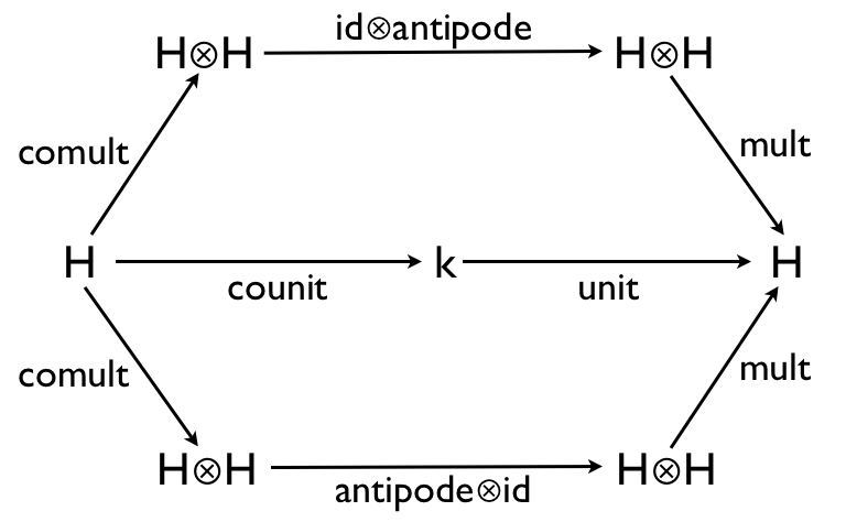
In particular,
mult . (id ⊗ antipode) . comult = unit . counit
Let's assume that an antipode for YSym exists, and see what we can deduce about it. The right hand side of the above equation is the function that takes a linear combination of trees, and drops everything except the empty tree. Informally:
(unit . counit) E = E
(unit . counit) (T _ _ _) = 0
For example:
> (unit . counit) (ysymF E) :: Vect Q (YSymF ())

F(E)

> (unit . counit) (ysymF (T E () E)) :: Vect Q (YSymF ())

0
Since we also know that comult E = E⊗E, and mult E⊗E = E, it follows that antipode E = E.
Now what about the antipode of non-empty trees? We know that
comult t = E⊗t + ... + t⊗E
where the sum is over all splits of t.
Hence
((id ⊗ antipode) . comult) t = E⊗(antipode t) + ... + t⊗(antipode E)
and
(mult . (id ⊗ antipode) . comult) t = E * antipode t + ... + t * antipode E
where the right hand side of each multiplication symbol has antipode applied.
Now, E is the identity for multiplication of trees, so
(mult . (id ⊗ antipode) . comult) t = antipode t + ... + t * antipode E
Now, the Hopf algebra condition requires that (mult . (id ⊗ antipode) . comult) = (unit . counit). And we saw that for a non-empty tree, (unit . counit) t = 0. Hence:
antipode t + ... + t * antipode E = 0
Notice that all the terms after the first involve the antipodes of trees "smaller" than t (ie with fewer nodes). As a consequence, we can use this equation as the basis of a recursive definition of the antipode. We recurse through progressively smaller trees, and the recursion terminates because we know that antipode E = E. Here's the code:
instance (Eq k, Num k, Ord a) => HopfAlgebra k (YSymF a) where

    antipode = linear antipode'

        where antipode' (YSymF E) = return (YSymF E)

              antipode' x = (negatev . mult . (id `tf` antipode) . removeTerm (YSymF E,x) . comult . return) x
For example:
> antipode $ ysymF (T E () E)

-F(T E () E)

> antipode $ ysymF (T (T E () E) () E)

F(T E () (T E () E))


> quickCheck (prop_HopfAlgebra :: Vect Q (YSymF ()) -> Bool)

+++ OK, passed 100 tests.
It is also possible to give an explicit definition of the antipode (exercise: find it), but I thought it would be more illuminating to do it this way.
It's probably silly, but I just love being able to define algebraic structures on pictures (ie of trees).
Incidentally, I understand that there is a Hopf algebra structure similar to YSym underlying Feynman diagrams in physics.
I got the maths in the above mainly from Aguiar, Sottile, Structure of the Loday-Ronco Hopf algebra of trees. Thanks to them and many other researchers for coming up with all this cool maths, and for making it freely available online.
> The binary trees we're concerned with are the familiar binary trees from computer science. In the math literature on this, however, they're called (rooted) planar binary trees. As far as I can tell, that's because in math, a tree means a simple graph with no cycles.
ReplyDeleteThe planarity requirement seems to be redundant here because it seems to be implied by the absence of cycles.
As it is stated by (Pontryagin—)Kuratowsky theorem the graph is not planar if it contains subdivisions of K_5 or K_{3,3} (cf. Wikipedia) which implies cycles. So no cycles — no K_5 or K_{3,3} — the graph (tree in our case) is planar.
Please, correct me if I'm wrong.
I think you're right that all trees are planar graphs. So I assume that "planar" as applied to trees has the implication that an embedding into the plane is given, and that it therefore makes sense to speak of one child node as being to the left or right of another, as seen from the parent node.
Delete